"Low-Latency Inference of Optimized AI-DSP Models for Hard Realtime Deadlines" by Christopher Johann Clarke (Singapore)
Digital audio processing is a hard real-time task. Each processing cycle must finish within a strict deadline set by the buffer size and sampling rate. If the deadline is missed, the result is an audible discontinuity. Unlike general-purpose computing, there is no allowance for variable execution time or occasional spikes in latency. Most current machine learning systems are designed for high throughput. They often rely on GPUs and parallel scheduling. These methods are effective for batch processing but do not address the timing requirements of real-time audio. In real-time contexts the worst case matters more than the average case. Operations that are acceptable in offline inference, such as asynchronous scheduling or dynamic memory allocation, cannot be tolerated inside a real-time audio process. This article describes strategies for running AI–DSP models under these conditions. It is divided into three parts: adjusting expectations to match fixed real-time limits, optimizing neural network structures to reduce computation and memory use, and implementing code that ensures bounded execution to support inference under the sub-millisecond deadlines common in current audio systems. I provide generic constructions of the arguments that I will be focusing on in the talk in this article.
Here is a plot of a single input inference, comparing the times for different models across different tasks
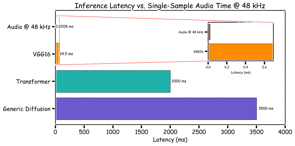
VGG16 https://keras.io/api/applications
Audio @ 48 kHz (1/48000 * 1000 = 0.0208 ms)
Optimizing our Expectations
As alluded to earlier real-time audio imposes fixed deadlines. Each processing block must be completed before the next buffer is required. This defines the maximum allowable computation per cycle. Any process that exceeds this bound produces failure in the audio stream. Neural models must be sized according to these limits. Large networks that operate in other domains cannot be used directly. Practical deployment requires reducing parameters, or some other method for reducing the amount of computation to be done. This has been shown by certain grey-box models to be effective. Research will continue to improve efficiency and enable larger models under the same deadlines, but when designing a system today the specification must reflect current hardware and software conditions. Planning should account for incremental improvements in the near term, but assuming hardware or framework advances years into the future is not viable for building reliable systems. The expectation is bounded execution time with minimal variance, defined by what is feasible at present and in the immediate future. All further stages of optimization assume this constraint as the baseline condition. To further use a line from Bencina (from “time waits for nothing”), we should consider an algorithm’s worst-case compute time instead of considering its averaged or amortised compute time.
Optimizing the Neural Network Architecture
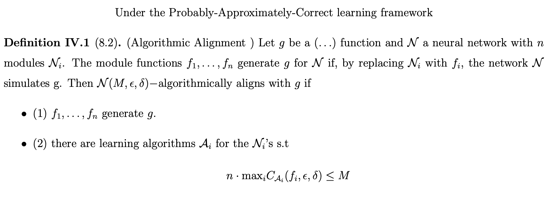
Once the external constraints are established, the network itself must be specified with respect to those constraints. Network design is often approached heuristically, through trial, error, or large-scale search. While this may eventually yield a working solution, it consumes resources and does not ensure suitability for real-time use. If we draw inspiration from Algorithmic Alignment, we can see that there should always exist some network for the function we want to achieve:
 As an example, we could run a grid search across many layers to find the ideal model size, but this takes time...
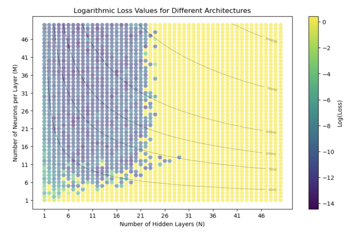
A more practical strategy is to define limits on model size in advance. This can be done by drawing on prior results, experimental evidence, or theoretical bounds, rather than relying solely on intuition. In practice, this may mean restricting the range of architectures to be tested, rather than attempting unconstrained grid searches across depth and width. For example, simple experiments (presented here at ADCx) demonstrate that searching across thousands of possible configurations can take days, while a bounded search guided by prior knowledge converges within the same order of accuracy in far less time . The aim is not to discover an optimum across the full space, but to establish a workable boundary within which models can be evaluated efficiently. I will present more of these optimizations at the talk. But by treating the network as a component subject to constraints, the design process becomes more predictable. The focus is no longer on achieving maximum performance without regard to cost, but on achieving sufficient performance while remaining within time and resource budgets. This approach reduces wasted computation, simplifies evaluation, and increases the likelihood that models trained in development can be transferred directly to deployment under real-time deadlines.
Optimizing the Code
General inference libraries are designed to maximize throughput or exploit large batch sizes. These choices are appropriate for offline or high-volume workloads but do not match the requirements of hard real-time audio, where latency per sample or per buffer is the primary constraint. RTNeural (github) was developed specifically with this use-case in mind. It is a lightweight C++ inference library intended for audio plugins and other systems with strict deadlines. Unlike larger frameworks, it does not assume batching, memory allocation during execution, or hidden scheduling.
Models can be built at compile time, embedding the architecture in the type system, or at run time using pre-exported weights.
// example of model defined at run-timestd::unique_ptr<RTNeural::Model<float>> neuralNet[2];// example of model defined at compile-timeRTNeural::ModelT<float, 1, 1,RTNeural::DenseT<float, 1, 8>,RTNeural::TanhActivationT<float, 8>,RTNeural::Conv1DT<float, 8, 4, 3, 2>,RTNeural::TanhActivationT<float, 4>,RTNeural::GRULayerT<float, 4, 8>,RTNeural::DenseT<float, 8, 1>> neuralNetT[2];
Both methods expose a simple per-sample forward() call that can be used directly inside the audio callback without additional overhead.
// in the processBlock()for (int ch = 0; ch < buffer.getNumChannels(); ++ch) {auto* x = buffer.getWritePointer (ch);for (int n = 0; n < buffer.getNumSamples(); ++n) {float input[] = { x[n] };x[n] = neuralNetT[ch].forward (input);}}
In practice, this means that initialization, weight loading, and memory allocation are done once, outside the callback. Execution inside the callback is reduced to deterministic state updates, with no blocking operations. Benchmarks included with the project show that RTNeural maintains real-time feasibility where general-purpose runtimes do not. For audio, this property is more important than absolute throughput, making RTNeural suitable as a code-level optimization for deploying learned models under hard deadlines.
Conclusion
Hard real-time audio requires bounded execution in every cycle. This work has outlined constraints on expectations, network design, and code implementation, showing how models can be made feasible under strict deadlines. The priority is not throughput but determinism; because in real-time audio, missing the deadline is not a slowdown, it is failure.