Ircam Forum Workshops

Despite the fact that a lot has already been said about granular synthesis, and the number of granular synthesisers may be counted in tens¹, in our opinion the potential of this type of synthesis is far from being exhausted. And while combining it with waveshaping with a certain design one can obtain some new sound results which could not appear in using just one of that kinds of sound synthesis.

1. Granular synthesis or ‘granulation’ ?

The idea of grains as small parts of sound signals was first proposed by Dennis Gabor² (Gábor Dénes), while the full theory and practice of granular synthesis was developed by Iannis Xenakis³. Later, Curtis Roads implemented its computer realisation⁴; Barry Truax further advanced the method, including its real-time realisation⁵.

Xenakis claimed in his lemma: ‘All sound is an integration of grains, of elementary sonic particles, of sonic quanta. Each of these elementary grains has a threefold nature: duration, frequency, and intensity’⁶. Today’s granular synthesis typically uses already existing sound to process, taking a small part of it as a grain and repeating it very fast, flexibly varying the characteristics of the repetition. To reduce grain density one can insert gaps between adjacent grains (see Section 7 for details); one of the solutions to make grain overlaps is using many ‘voices’ of grain repetitions. 

So where is the border between synthesis and ‘granulation’ or just ‘processing’? Since which point the granular method really synthesise new sound instead of just montaging the existing one? In our view, a synthesis starts when we no more hear the source sound, but the new sound with new parameters is generated (and that means that for us most of commercial granulators are not synthesisers, but rather ‘texturisers’). 

Since we’re using a pre-recorded sound with already existing frequency and spectrum (and setting aside issues of intensity for a while) we need to rework our approach to Xenakis’ lemma three parameters. Our GranShaper project takes following three main parameters for granular synthesis:

• frequency of repetition of the grain [𝑓, Hz];
• playing rate — does the grain is being played back at original rate 1:1 or faster/slower? [𝑟, times];
• grain time position (time offset) in the source sound [𝜏₀, seconds].

One cannot control the source sound’s grain length (or duration: 𝑙) as it completely depends on and calculates from the first two parameters: 

𝑙 = 𝑟 : 𝑓        (1)

On lower repetition frequencies we perceive a repetition frequency as a tempo of an ostinato; we hear the pitch of an original sound and a playing rate transposes it. We recognise the source sound. But if the frequency is above 20 Hz we no more hear the source; frequency becomes new pitch, and original pitch altered by playing rate becomes formant of the new sound (see Fig. 1). This is a moment when the real synthesis starts.

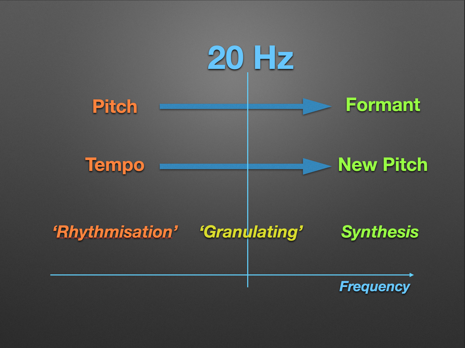
  Fig. 1. Changing perceived sound parameters depending on repetition frequency

Probably, the first brilliant example of such quality changing while crossing the border of 20 Hz is given in Kontakte (1958—1960) by Karlheinz Stockhausen.

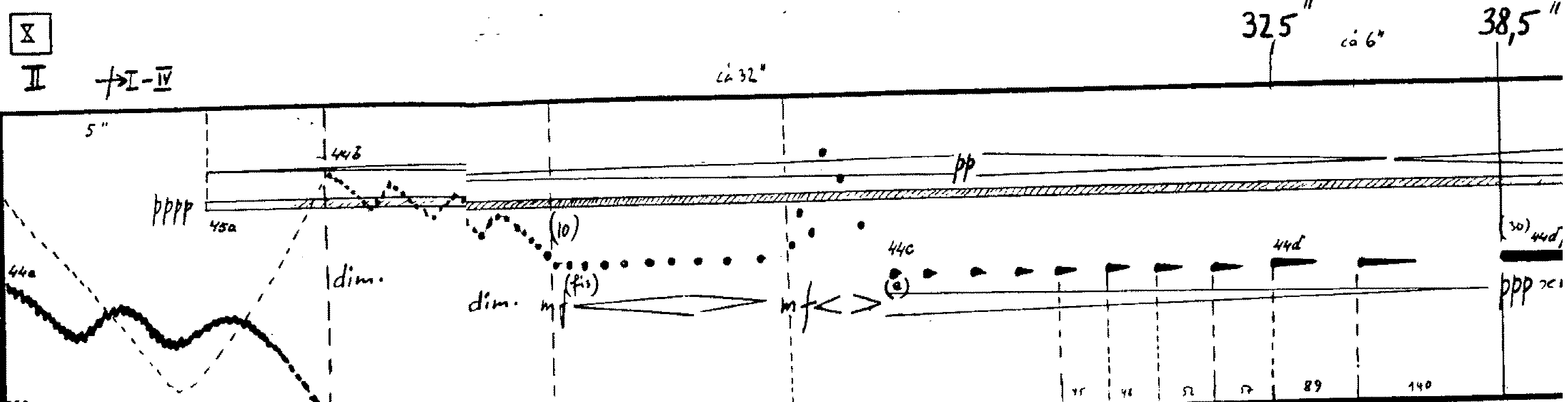
Fig. 2. Karlheinz Stockhausen. Kontakte. Section X. L.: Universal Edition, 1966. P. 19–20

Usually, this work is not counted as a granular synthesis example because there is neither pre-recorded sound nor chaotisation used, which is commonly considered characteristic of granular synthesis. But actually, Stockhausen used a granular technique here: a very short sound which was created before is being repeated very quickly, and its repetition frequency forms the new pitch. It makes vast downward glissando, and the first vertical dashed line in the score (see Fig. 2) shows the point where this slide crosses the border of 20 Hz, moving us from sound synthesis to rhythmisation or from the pitch area to the rhythm area according to Stockhausen’s terms⁷. After crossing this threshold we realise that this low sound with rich spectrum actually is a sequence of very short sine pieces with high pitch. 

2. Granular ‘vocoder’

Above we touched on the role of parameters Nos. 1 (repetition frequency) and 2 (playing rate), but said nothing about 3rd parameter, the time position of the grain. Perhaps, the most interesting feature of granular synthesis is the dynamic aspect of its parameters: diverse strategies of continuous changing the values results in vast variety of complex sounds, which was primarily demonstrated in the first ‘official’ precedent of granular synthesis, Analogique B (1958—1959) by Iannis Xenakis⁸. When all parameters are enough stable (the values changes very slowly) and 𝑓 > 20 Hz, the resulting signal is close to be periodical and the sound is close to a tone. In GranShaper one can play melodies and chords by such tones (particularly using a MIDI keyboard). But when values are in dramatic changing, the sound is no more periodical, so we obtain different kinds of noises and transitional sounds. 

Particularly, while our time position (𝜏₀) is grading continuously, we can hear different parts of original sound in granularly transformed way. When 𝜏₀ increases from the beginning to the end with a speed close to normal playback speed, the obtained sound most closely resembles the source sound because the process of its playing mostly reminds normal playback. The difference is that instead of just playing it from the beginning to the end (how denoted in Fig. 3) 

Fig. 3. Simple playback (time axis)

we play it zigzag way by small pieces and every next piece (grain) starts from the later time point 𝜏₀ (Fig. 4).

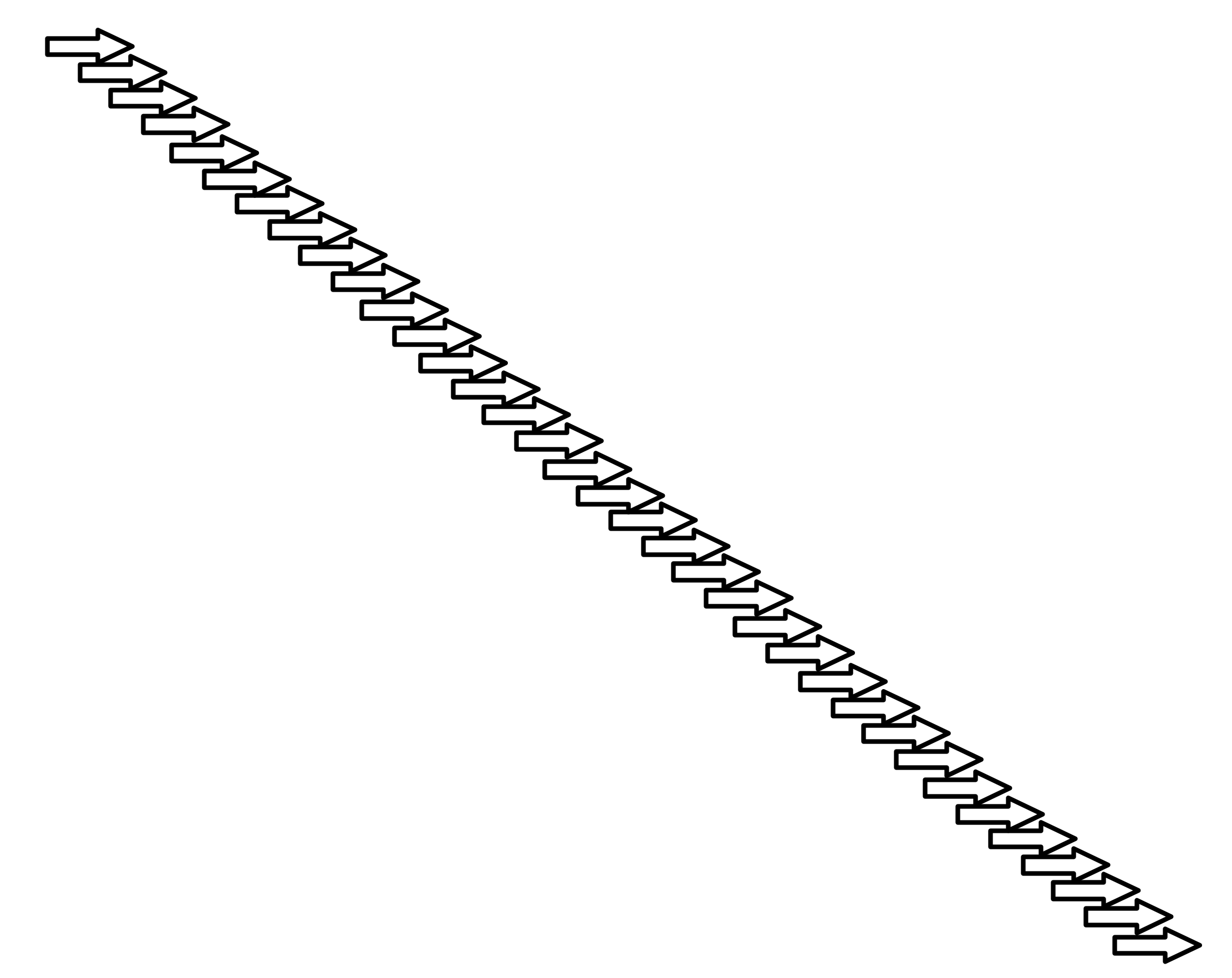
Fig. 4. Granular ‘playback’ with continuously increasing grain starting position 𝜏₀

 The resulting sound is still a tone as it has a structure which is very close to periodical: every grain is its period since the neighbour grains are very similar (as far they started from not the same but very similar time point from the source sound)—thus their sequence forms quasiperiodical signal. On the other hand the result strongly resembles the source sound as we ‘scan’ it from the beginning to the end which reminds simple playback. 

So the sound we obtain is ambivalent and possesses qualities of both source sound and new tone. We call this effect granular ‘vocoder’. Indeed this is not real vocoder as it doesn’t use any frequency domain technique. It sounds differently, but sometimes reminds vocoder processing. One can even use it in typical vocoder situation if loads some speech example as a source sound, takes a chord and slides ‘starting position’ (𝜏₀) slider slowly from the beginning to the end. The chord will start ‘speaking’.

Interesting feature of this technique is that we can modulate from the tone (or chord) to the original sound by altering the speed of changing 𝜏₀: where this speed is exactly equal to normal playback speed, the end of the previous grain is exactly the same moment (in the source sound) as the beginning of the next one. So, ideally it ‘degenerates’ into just normal playback (Fig. 5).

Fig. 5. Granular playback ‘degenerates’ into normal playback when 𝜏₀ is exactly equal to normal playback speed.

That said, we should mention that this is true only when the playing rate (𝑟) is normal 1:1. Then we can generalise our statement: where the speed of 𝜏₀ changing is exactly equal to 𝑟, the end of the previous grain is exactly the same moment (in the source sound) as the beginning of the next one. So, ideally it ‘degenerates’ into just normal playback with 𝑟 rate (when 𝑟 is not 1, the source sound is transposed and stretched/shrinked).

However when the speed of 𝜏₀ changing is very slow, we hear the tone (or chord) but not the source sound. In the case when the speed of 𝜏₀ changing is less that 𝑟 but doesn’t approach to 0, we hear the ‘vocoder’ effect, because the tone is ‘coloured’ by the source sound. And when the speed of 𝜏₀ changing is much more than 𝑟 or quite less than 0 (so we move back) we hear quite different complex sound. So by modulating that speed from 0 to 𝑟 and further we can perform a transition between the new tone (or chord) to the source and, further, to other kinds of sound. 

3. Granshaping

‘Granular waveshaping’ is a kind of hybrid of the two types of synthesis mentioned in its name. 

3.1. Two perspectives on waveshaping.

Generally, waveshaping is a non-linear interaction of two signals. This kind of synthesis was discovered by Daniel Arfib⁹ and Marc Le Brun¹⁰ in 1978–1979.

In common DAW context, waveshaping is understood as a kind of sound processing which remaps the values of the input signal according to a second signal as a mathematical function. Using this approach we treat an input signal as a sound and the second signal as a transfer function. Thus, waveshaping is treated as a kind of complex amplification of an input. This point of view allows us easily describe and model such non-linear processing devices as overdrive, distortion, saturation etc. (and such waveshaping description was historically the first).

But quite other approach to waveshaping is possible as well. We can also perceive the second signal as a pre-recorded or generated sound and the input signal as a control which drives the phase of playing the second signal. From this position waveshaping is thought of as complex changing of playback time of the previously sampled sound: the input signal now controls a ‘playback cursor’ for the loaded sound.

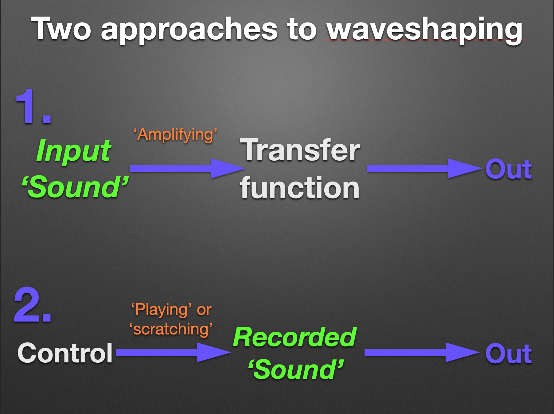
Fig. 6. Two approaches to waveshaping

Consequently we can treat both control and transfer signals as sounds altering one another in waveshaping process. When we focus on the first sound we see how the transfer changes its values; and when we focus on the second sound we can observe how the control alters its phase or, better say, playback trajectory. Both explanations are equally valid and describe the same thing (Fig. 6).

3.2. Granshaping as a ‘doubled’ granular synthesis.

So, if both signals can be sounds, we will consider them as such. Granshaping is a synthesis where both of these signals are synchronised grains of two different source sounds. Both grains have their individual playing rate (𝑟) and time position (𝜏₀) values but the repetition frequency (𝑓) is the same as the grains are synchronised. As a result, ‘granular waveshaping’ is like granular synthesis ‘multiplied by two’: both sounds have independent settings, for example for randomisation.

Technically, GranShaper is developed in the Max/MSP programming environment¹¹ as a Max project, utilising the gen extension¹² for sound processing operations (gen~ object). Since our granular engine is implemented as a basic chain of Max gen objects — ‘phasor → (scaling) → peek’ — our granshaping engine extends this structure with an additional step: ‘phasor → (scaling) → peek → (scaling) → another peek’.

The result is intensely energetic sound with incredibly rich spectrum.

Here the parameters of granular synthesis can get a new interesting interpretation. The control’s both amplitude and formant (altered by playing rate) affects to shifting resulting sound spectrum higher or lower (but with different nuances). 

Sometimes it makes sense using extremely low playing rate for one of the two grains as even using very short grain is enough to create a very saturated sound. When we dramatically reduce playing rate of one of two source sounds, we use grains of very different sizes: one is ‘middle’ and another one is extremely short. In this case our ‘two approaches’ to waveshaping are applicable practically; this is most clear on low frequencies. When our transfer grain is quite shorter than the control grain, we can use ‘approach 1’ i. e. our sound reminds the first source sound ‘processed’ by the second one: the result sounds close to non-linear effects like distortion. And when we, vice versa, take the control grain very short and transfer is quite longer, the ‘approach 2’ better describes the situation: our sound looks like DJ scratching, when the second sound is ‘scrubbed’ or ‘rewinded’ while playing back.

On the frequencies above 20 Hz the results will be various sounds with huge variety of harmonically rich spectrum.

4. Granular Shapemorphing

Let’s turn back to waveshaping however. If one of the two signals is a ramp (linear function), the result of waveshaping is similar to the other signal. For example when the control is a linear function, that means that the transfer is just being played from the beginning to the end with a constant speed. Actually it turns to what the phasor object does. At the other hand, when the transfer is a ramp any input value is just equal to output one, i. e. the control is just bypassed. Consequently, ramp signal in waveshaping is kind of ‘default’ signal which changes nothing. 

Thus, 

waveform 1 → ramp = waveform 1               (2)

ramp → waveform 2 = waveform 2

where ‘→’ is waveshaping.

We took advantage of this feature by creating a mix of a ramp and some other wavetable in different proportions for each of the interacting granules. By such crossfade between the ramp and a certain wavetable, we change a contribution of this waveform into a synthesis. This trick allows smooth transformation from one sound to the other, from signal 1 to signal 2. When one of them turns to the ramp we just hear another. When we use both source signals without mixing with a ramp we generate a waveshaping sound which is quasi ‘in the middle’ of the source sounds but it is actually not the ‘middle’ but quite more energetic than the original signals. Because of the non-linearity of the waveshaping processes, the resulting intermediate sounds could not be simply referred as a mix. We described this process as ‘granular shapemorphing’.

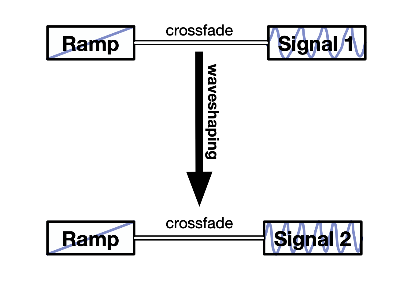
Fig. 7. ShapeMorphing algorithm allowing gradual transition between the control and the transfer via using crossfades with ramps

The construct depicted on Fig. 7 can assume the following extreme states (Fig. 8):

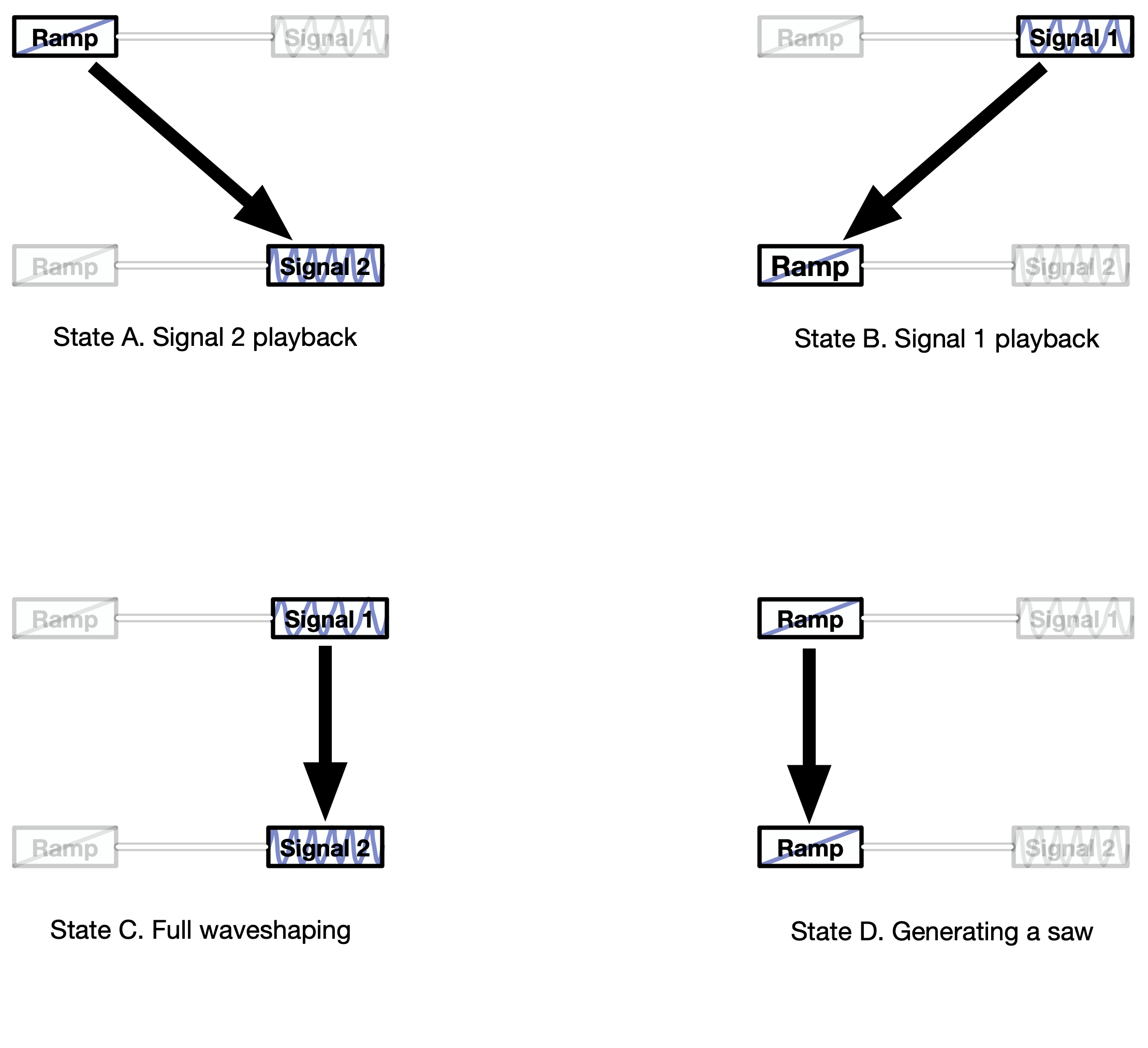
Fig. 8. Extreme states of ShapeMorphing engine, when the output is:
A. Transfer signal; B. Control signal; C. Product of real waveshaping; D. Just saw waveform 

All possible intermediate states provide what we could refer as ‘morphing’—in quotes indeed, because it is, like our ‘vocoding’, neither a spectral technique nor a simple crossfade between two sounds A and B (so it’s not a real morphing in a traditional sense). In our scheme, the crossfades are used to make gradual transitions between waveshaping and ‘clean’ sound and the intermediate sound between the source waveforms A and B is a waveshaping product С which is actually not ‘in between’ of them two.

Thus, our method of sound transitions forms a 2D space represented by a pictslider in GranShaper. It’s depicted on Fig. 9:

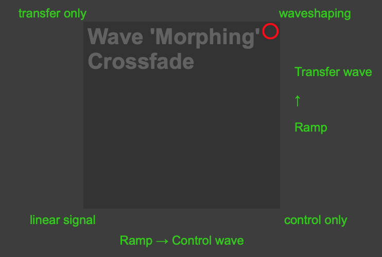
Fig. 9. Fragment of GranShaper interface: pictslider object for manipulating ‘moprhing’

5. Mathematical details

It would make sense to include above all the the formulae, but since this article is intended for musicians, we chose not to overload it with mathematical expressions. However, it would still be worthwhile to provide a mathematical description of all the processes outlined here.

5.1. Formula for our granular synthesis method

(without randomisation and other parameters changes):

𝑠 (𝑡) = 𝑔 ( 𝜑(𝑓𝑡) • 𝑟 / 𝑓 + 𝜏₀)             (3)

where:

• 𝑠(𝑡) is the resulting signal,
• 𝑔(𝜏) is the source signal (𝜏 represents the time of the recorded source signal, technically the sample number, as opposed to 𝑡, which is the real time of the resulting sound),
• 𝑓 is the repetition frequency in Hz,
• 𝑟 is the playback speed, defined as 𝑙 •𝑓, where 𝑙 is a grain length (see formula (1)), being the difference between 𝜏_m and 𝜏₀, where 𝜏_m is the end of the grain, a temporal position in the source sound corresponding to the playback end, while 𝜏₀ is the start of the grain,
• 𝜑(𝑓𝑡) is the phase, normalised to range 0…1, as a function of time 𝑡, scaled by the repetition frequency 𝑓 (actually, the Max’s phasor object function);
  so 𝜑(𝑓𝑡) / 𝑓 represents the time ‘wrapped’ to a single grain.

The full formula without ‘𝑟’ looks like follows:

𝑠 (𝑡) = 𝑔 ( 𝜑(𝑓𝑡) • 𝑙 + 𝜏₀) = 𝑔 ( 𝜑(𝑓𝑡) • (𝜏_m – 𝜏₀) + 𝜏₀)          (4)

To this formula, various randomisations and parameter modifications are to be added. 

5.2. For example, for granular ‘vocoding,’

gradual modification of the initial playback position 𝜏₀ is necessary. If 𝜏₀ changes from the beginning to the end at a normal playback rate, then:

𝜏₀ = 𝛱 • ⌊𝑡/𝑃⌋             (5)

where:

• 𝛱 is the ‘period’ inside the internal time 𝜏 of the recorded sound, i. e., the temporal distance between the starts of two adjacent grains within the source sound (for normal playback speed, 𝛱 = 𝑃, then 𝜏₀ is close to 𝑡),
• ⌊ ⌋ denotes rounding down to the nearest integer (truncating), ensuring that 𝜏₀ changes discretely, once per period (to prevent changes in 𝜏₀ from affecting the actual grain playback speed). Technically, this rounding is performed by the sah (‘sample-and-hold’) object in Max gen and MSP.

So, the general formula for playback in granular ‘vocoding’ is

𝑠 (𝑡) = 𝑔 ( 𝜑(𝑓𝑡) • 𝑟 / 𝑓 + 𝛱 • ⌊𝑡/𝑃⌋)          (6)

5.3. The granshaping formula

represents a ‘doubling’ granular synthesis. Here, 𝑔(𝜏) is the already familiar granular synthesis function representing the control, while 𝑘(𝜏_k) is a similar granular synthesis function applied to a different pre-recorded sound representing the trasnsfer, where its playback parameters (rate 𝑟_k and initial grain start time 𝜏₀_k) can be set independently:

𝑠 (𝑡) = 𝑘 ([½ 𝑔 ( 𝜑(𝑓𝑡) • 𝑟 / 𝑓 + 𝜏₀) + ½] • 𝑟_k + 𝜏₀_k)              (7)

Manipulations with ½ are just scaling the control signal 𝑔 (𝜏) from –1…1 to 0…1 range to be valid for ‘phasing’ the transfer signal 𝑘 (𝜏_k).

5.4. GranShapeMorphing.

The formula below generalises the previous formula (7) by including a ramp 𝜑(𝑡) — its value is equal to phase (normalised to the range 0…1; technically we mix the phasor output to the sound) — and crossfading signal weights 𝐴 (for the control) and 𝐴_k (for the transfer):

𝑠 (𝑡) = 𝐴_k • 𝑘 ([½ 𝐴 • 𝑔 ( 𝜑(𝑓𝑡) • 𝑟 / 𝑓 + 𝜏₀) + ½] • 𝑟_k + (1–𝐴) • 𝜑(𝑓𝑡) + 𝜏₀_k) + 
+ (1–𝐴_k) • 𝜑 ([½ 𝐴 • 𝑔 ( 𝜑(𝑓𝑡) • 𝑟 / 𝑓 + 𝜏₀) + ½] • 𝑟_k + (1–𝐴) • 𝜑(𝑓𝑡) )               (8)

Indeed this is a cumbersome formula, but it can be simplified by introducing a substitution:

([½ 𝐴 • 𝑔 ( 𝜑(𝑓𝑡) 𝑟 / 𝑓 + 𝜏₀) + ½] 𝑟_k + (1–𝐴) • 𝜑(𝑓𝑡) ) = 𝐦                         (9)

where 𝐦 represents a ‘mixed input’ — a weighted sum of the control signal 𝑔(𝜏) and the ramp 𝜑(𝑡). Then:

𝑠 (𝑡) = 𝐴ₖ • 𝑘 (𝐦 + 𝜏₀_k) + (1–𝐴_k) • 𝜑 (𝐦)                           (10)

6. Randomization

Admittedly, granular synthesis has been inconceivable without statistical and probabilistic procedures. While formulating the principles of granular synthesis, Xenakis introduced the concepts of ataxy (order or disorder) and of cloud of grains¹³. In GranShaper, we use four kinds of randomisation for each of three main parameters — grain repetition frequency (𝑓), playing rate (𝑟) and grain time position (time offset; 𝜏₀):

• ‘dispersion’, i. e. parameter range, Δ (units depend on the parameter);
• frequency of parameter change, ‘tempo’, 𝐹 (Hz; values like 1000 Hz could be understood as ‘continuous change’ as we cannot hear events more often than 20 times per seconds; all values below forms a constant rhythm of changes);
• ‘dispersion’ of changing frequency, i. e. tempo range of frequencies of the parameter changes or ‘tempo range’; it could be also called ‘rhythmic acuity’ or ‘durations contrast’, because this parameter makes a transition between equal rhythm of changes to a rhythm with very different durations, Δ𝐹 (octaves);
• frequency of change of diffusion of frequency of changing a parameter: with the high values of this variable the ‘rhythm’ changes in every unit, but with the low values it could changes rarely, allowing sequence with same durations in a row, also ‘rhythm irregularity’, 𝐼 (Hz).

We use Max noise object to generate random signal in a range –1…1. So, let 𝛕₀, 𝒇, 𝒓, 𝑭 are respectively time position, repetition frequency, playing rate and frequency of a parameter changes after randomisation while 𝜏₀, 𝑓, 𝑟, 𝐹 are the same parameters before randomisation (parameters being set); ‘noise’ is a function of time 𝑡 scaled by 𝑭 or 𝐼 and quantised by ⌊⌋ with sah object for preventing changes within a grain to avoid distortions.  

Then the final time position is:

𝛕₀ (𝑡) = 𝜏₀ + noise (⌊𝑭_𝜏 𝑡⌋) • Δ𝜏₀                             (11)

𝑭 _𝜏(𝑡) = 𝐹_𝜏 • 2 ^ (noise (⌊𝐼_𝜏 𝑡⌋) • Δ𝐹_𝜏)         (12)

the final repetition frequency:

𝒇 (𝑡) = 𝑓 • 2 ^ (noise (⌊𝑭_𝑓 𝑡⌋) • Δ𝑓 )                        (13)

𝑭_𝑓 (𝑡) = 𝐹 • 2 ^ (noise (⌊𝐼_𝑓 𝑡⌋) • Δ𝐹_𝑓 )          (14)

the final playing rate:

𝒓 (𝑡) = 𝑟 • 2 ^ (noise (⌊𝑭_𝑟 𝑡⌋) • Δ𝑟)                           (15)

𝑭_𝑟(𝑡) = 𝐹_𝑟 • 2 ^ (noise (⌊𝐼_𝑟 𝑡⌋) • Δ𝐹_𝑟)           (16)

7. Windowing: overdrive and ‘staccato’

A common solution for avoiding clicks on the grain borders is multiplying the grain to a window function to create fade-ins and fade-outs¹⁴. We apply very common von Hann window¹⁵ for that purpose. 

But for our taste, ordinary windowing sometimes makes granular sound too sterile, causing it to lose some of its raw energy—energy that is preserved in the Kontakte example in Fig. 2. Clicks or transients at grain borders contribute to the sound spectrum, making it richer when 𝑓 rises above 20 Hz. To preserve both the possibility of using a standard Hanning window and approaching a rectangular one, while nonetheless avoiding clicks at lower frequencies, we apply overdrive to our window by multiplying it by a coefficient and transforming it with a hyperbolic tangent. This operation ‘fattens’ the window, making the fades shorter, but they never disappear, as the hyperbolic tangent is a smooth function (see Fig. 10). This witty solution has been suggested by composer and media artist Alex Nadzharov¹⁶.

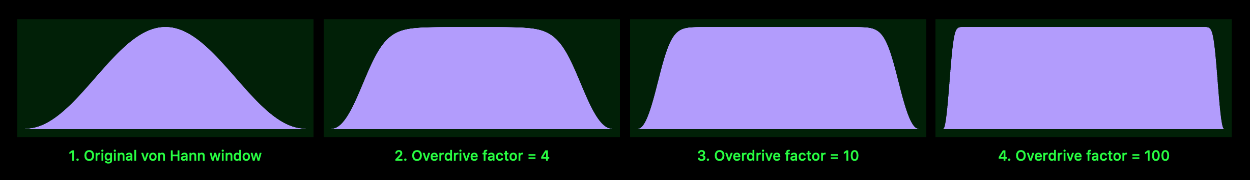
Fig. 10. Von Hann window overdriven by hyperbolic tangent with different scaling before

The other kind of window transformation creates a ‘staccato’ effect, where a grain is cut off before reaching its full duration. At lower frequencies, this produces a true staccato, while above 20 Hz, it results in a ‘thinner’ sound with a redistribution of spectral energy towards higher frequencies. Technically, this effect is achieved by accelerating the window playback, so it reaches its end before the grain is fully played, causing the remaining part of the grain to be silenced.

Finally, windowed sound with applied combination of window overdrive and ‘staccato’ can be expressed as follows:

𝑤 (𝑡) = 𝑐 • tanh [𝑎 • Hann (𝑞𝑡)] • 𝑠 (𝑡)                 (16)

where:

• 𝑤(𝑡) is windowed sound,
• 𝑎 is an overdrive coefficient (overdrive factor),
• 𝑐 is a certain amplitude compensation after applying tanh (which reduces sound level on low 𝑎 values),
• Hann(𝑡) is the von Hann window function (we store it pre-generated in a buffer, so we don’t need to calculate this function every time),
• 𝑞 is ‘staccato’ window playing accelerator: as it equals to 1, there is no ‘staccato’—the window is being played full grain length; the higher the value, the faster the window is played, shortening the actual duration of the grain,
• 𝑠(𝑡) is unwindowed signal (obtained by formulas (8), (10) + randomisation).

8. ‘MMMM’

Technically, the GranShaper is implemented within the ‘MMMM’ format, which we designed. It provides a standard framework for building flexible, microtonal synthesisers within Max-MSP, controllable via MIDI. Actually, ‘MMMM’ (‘Max MIDI Music Microtonal’) is a standardised Max patch where one can put their own synthesiser engine without worrying about polyphony, MIDI control, or microtonal pitch remapping (as shown on Fig. 11). The MMMM patch:

• processes MIDI polyphony, making it work like a traditional keyboard-controlled synthesizer;
• handles microtonal pitch mapping, computing frequencies for non-12 TET tuning systems;
• provides flexible MIDI control, including pitch bend and modulation wheel, with adjustable range settings;
• expands sustain pedal functionality, offering four distinct modes, including sostenuto.

The key advantage of ‘MMMM’ is simple integration: any oscillator or synthesis engine can be inserted into this framework, instantly gaining all these advanced MIDI features without requiring additional programming. This allows for rapid development of diverse synthesisers, all sharing a unified control interface.

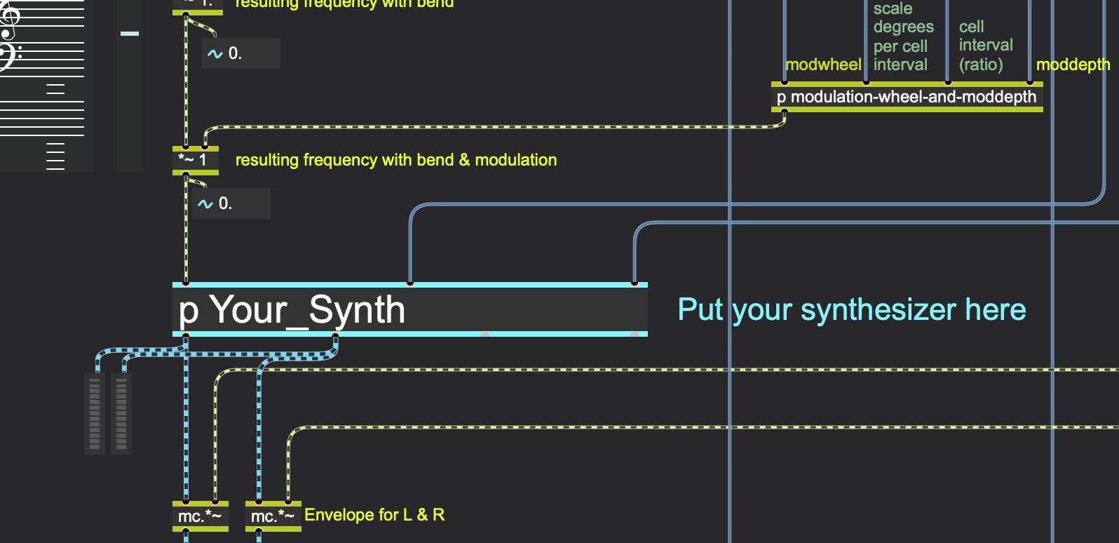
Fig. 11. ‘MMMM’ subpatch for putting a new synthesiser engine into standardised interface

For GranShaper, ‘MMMM’ provides ‘normal’ polyphony, but inside each voice, we introduce a multitude of grains. Thus we can play either ‘normal tones’ (with ‘MMMM’ microtonal and MIDI keyboard tools) or all granular and shaping features: textures, probability, complex repetitions, overtone glissandi, timbre transitions etc.

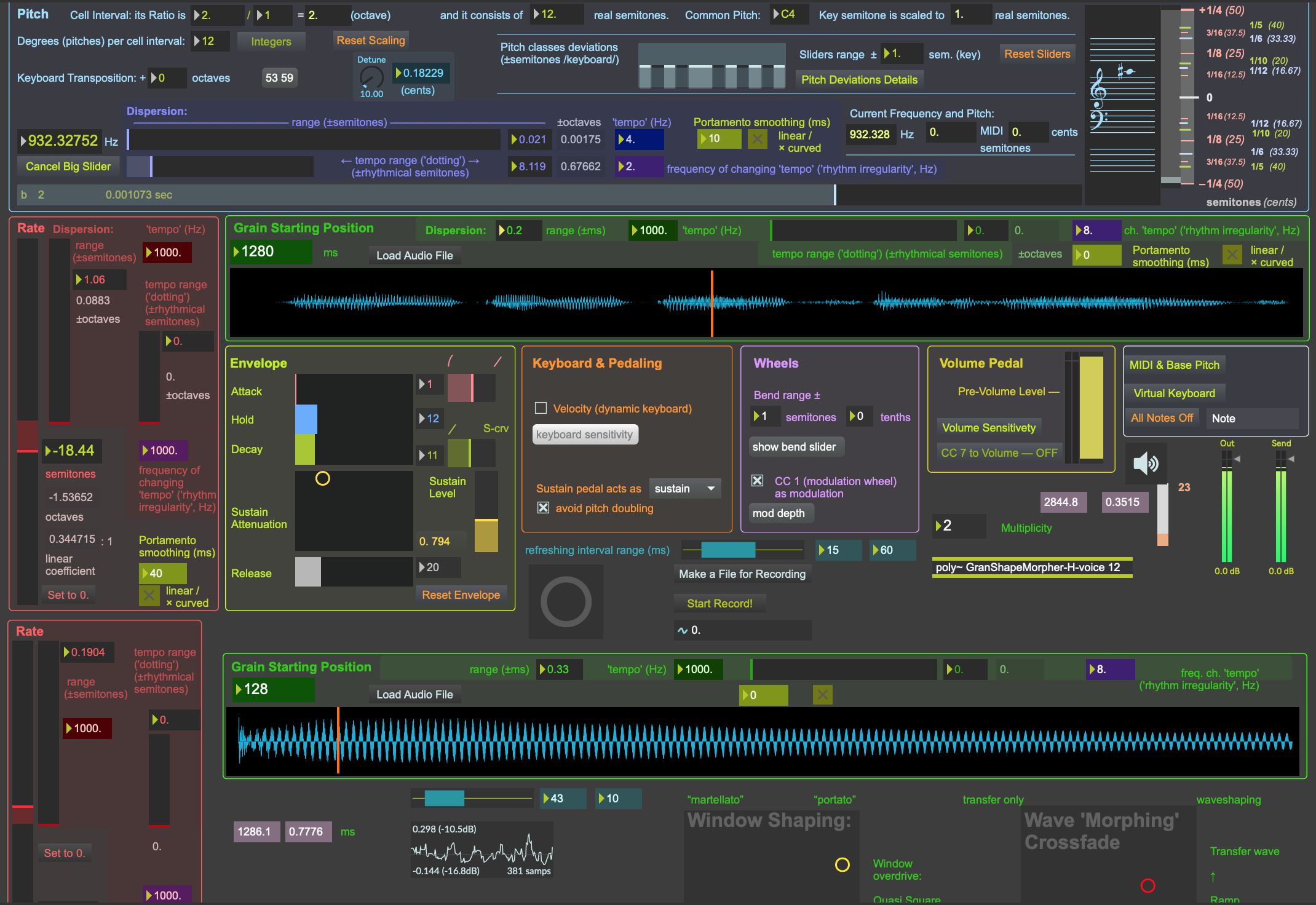
Fig. 12. GranShaper interface fragment

‘MMMM’ is still in progress, but we hope that in the future it will enable the creation of an open community of developers who will contribute new synthesisers within this framework and help build a large open library. As ‘MMMM’ simplifies making interface, polyphony and all MIDI stuff, it will allow for faster creation of new synthesisers. 

Conclusion

In this article, we began our exploration with well-known concepts such as granular synthesis and waveshaping in general, but we also introduced our own perspective on these topics. Building on these foundations, we proposed and described several new approaches to sound synthesis and sound processing techniques, including granular ‘vocoding’, granshaping, and granshapemorphing. Finally, we presented their technical implementation in Max as the GranShaper synthesizer, based on the ‘MMMM’ format.

GranShaper is still a work in progress—we have much testing and refinement ahead. Thus, this article serves more as a presentation of new synthesis strategies and principles rather than a finalised product. Stay tuned for updates and announcements regarding GranShaper and ‘MMMM’.

Notes

¹ Here are just a few examples: Monolake Granulator by Robert Henke (Max-for-Live Device) — https://www.ableton.com/en/packs/granulator-ii/, Borderland Granular by Chris Carlson — http://www.borderlands-granular.com/app/, Crusher-X by AccSone — https://accsone.com, grainflow, LowkeyNW, and petra (by Circuit Music ) for Max — see Max Packages. Meanwhile, commercially driven online music resources are full of titles like ‘17 Best Granular VST Plugins’ (e. g., https://www.musicindustryhowto.com/granular-vst-plugins/).

² See Xenakis (1992, 54, 58, 103, 373); Roads (2001, 22, 27–28).

³ See Xenakis (1992, 43–109); Roads (1996, 196).

⁴ See Roads (1996, 196).

⁵ See ibid.

⁶ Xenakis (1992, 43).

⁷ See Stockhausen (1957, 10–40).

⁸ See Xenakis (1992, 103–109).

⁹ See: Arfib (1978), (1979, 757–768)

¹⁰ Le Brun (1979, 250–266).

¹¹ See https://cycling74.com/products/max.

¹² See https://docs.cycling74.com/legacy/max8/vignettes/gen_topic.

¹³ See Xenakis (1992, 63–68, 182, 12).

¹⁴ See Roads (2001, 87–90).

¹⁵ On the von Hann function, see: Blackman, Tukey (1958, 200–201).

¹⁶ See Alex Nadzharov’s website: http://alexnadzharov.com/.

References

1. Arfib, Daniel. Digital Synthesis of Complex Spectra by Means of Multiplication of Nonlinear Distorted Sine Waves. Proceedings of the 1978 International Computer Music Conference (ICMC), 1978. https://quod.lib.umich.edu/i/icmc/bbp2372.1978.009/1.
———. Digital Synthesis of Complex Spectra by Means of Multiplication of Nonlinear Distorted Sine Waves. Journal of the Audio Engineering Society 27, no. 10 (1979):
757–768. https://aes2.org/publications/elibrary-page/?id=3178.

2. Blackman, R. B., Tukey, J. W. The Measurement of Power Spectra from the Point of View of Communications Engineering – Part I. Bell System Technical Journal 37, no. 1 (January 1958): 185–282. https://archive.org/details/bstj37-1-185/page/n15/mode/2up.

3. Le Brun, Marc. Digital Waveshaping Synthesis. Journal of the Audio Engineering Society 27, no. 4 (1979): 250–266.

4. Roads, Curtis. Computer Music Tutorial. Cambridge, MA: MIT Press, 1996. https://mitpress.mit.edu/9780262680820/the-computer-music-tutorial/.

5. Roads, Curtis. Microsound. Cambridge, MA: MIT Press, 2001. https://mitpress.mit.edu/9780262681544/microsound/.

6. Stockhausen, Karlheinz. …how time passes… Die Reihe 3 (1957): 10–40. ISSN 0486-3267.

7. Xenakis, Iannis. Formalized Music: Thought and Mathematics in Composition. Edited by Sharon Kanach. Hillsdale, NY: Pendragon Press, 1992.
https://www.pendragonpress.com/formalized-music.html.